Bird Detection TinyML

This article covers the creation of a localized bird detection machine learning model. There are, of course, solutions that rely on internet connectivity to perform a more accurate examination based on a provided image but this model approach could allow for low powered, long lasting, tracking at the edge.

Note: I’m self taught. Take my musings with a grain of salt.

Models

The following models have been generated as part of this research / work. The models are being released here along with some information below about how they were generated. Releasing them for non commercial use. I’m also up for discussing partnerships if there’s a particular model that needs to be shrunk or if anyone wants to discuss funding additional research.

• Dataset: BIRDS 525 SPECIES- IMAGE CLASSIFICATION
• Data Preparation Notebook: birds_data_prep.ipynb

The data preparation notebook above loads up the training folder of the above dataset, creates train, validation, test splits, and then further defines a bird feeder birds subset and copies just these birds to another set of folders to be used while training the 411 reduced output set.

Image Size	Activation	Outputs	Parameters	Accuracy (Quantization)	Download
224x224	Swish	524	4,491,895	95.31%	Notebook - Model
96x96	Swish	524	4,491,895	89.91%	Notebook - Model
96x96	Partial Relu	524	4,491,895	89.74%	Notebook - Model
96x96	Relu	524	4,491,895	89.91%	Notebook - Model
96x96	Relu	524	746,263	80.14%	Notebook - Model
96x96	Relu	524	196,533	82.03%	Notebook - Model
96x96	Relu	411	190,770	85.05% (74.16%)	Notebook - Model
88x88	Relu	411	190,770	84.04% (74.84%)	Notebook - Model
80x80	Relu	411	190,770	82.67% (72.85%)	Notebook - Model
80x80	Relu6	411	190,770	81.4% (79.44%)	Notebook - Model
96x96	Relu6	411	190,770	83.49% (82%)	Notebook - Model

The models are ordered in the order of their creation.

In addition the final model’s quantized tflite is available here along with a labels.txt file with a comma separated label list. In addition I’ve added an Edge Impulse Project with the uploaded tflite model and labels to make downloading easier.

Note: int8 quantization is very picky when it comes to activation choice. Using relu helps from my experience but it wasn’t until I switched to relu6 that I saw consistent results more in line with the prequantization. Swish results generally were poor with the int8 quantization. Relu was highly influenced by representative dataset where relu6 was not; I saw larger swings between reruns of quantization in the 10-15% range while for relu6 I saw only around a percentage point change between reruns (I reran quantization several times to attempt to get a good representative dataset – something I feel I still need to improve my process toward).

Background

Last fall I took interest in the ITU’s TinyML contest around creating a TinyML based animal detection model to fit on smaller hardware. At the time I knew nothing of machine learning and struggled to get high accuracy in the model I created. I later tried using transfer learning via MobileNet which helped my accuracy but it became clear to me that these base models were designed for much larger hardware. I began experimenting by removing layers from my model but ran out of time before the deadline.

With the defeat from the ITU TinyML competition I was disheartened but still interested in machine learning and seeing if I could come up with some feasible way to shrink these larger models. Looking for motivation I decided I’d work on a bird feeder bird identification project as I figured there would be high quality datasets, a strong interest in the subject from the community, and it would challenge me with a large number of outputs which otherwise may be difficult to fit on smaller hardware. I found a dataset with a permissive license, trained the model in the traditional transfer learning way, and began experimenting.

Careful: The author of the dataset included a joke category called “Looney Birds” which includes various humans. Also at least a subset of the images appear to been obtained from sites that watermark their images leading one to question whether the dataset author is licensed to distribute them.

Though I encountered multiple difficulties in the process I eventually was able to compress the model to the size to fit on smaller devices while still retaining most of its accuracy. This model couldn’t be used though on my devices as the RAM requirements from a 224x224x3 input model were far too large. I kept at it and was able to rework the model to a smaller input size. My excitement quickly soured as I realized the default test segment had only five images per bird so I couldn’t confidently say the model would work well in the wild. I had to restart and this time use a proper spread of train to test data.

This article is the conclusion of that process. It took several months to get to this point and requiring refinement of various techniques along the way. I am documenting some elements of it here and releasing associated models at various stages of the compression.

I’m not sure if there’s a significant flaw to my approach in any way. When I’ve tried recent (to avoid catching ones the dataset author may have included) random images of birds on the model I’ve found it properly categorized most of them (and those it didn’t I could see the resemblance).

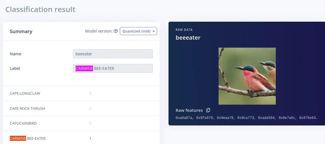
For example: I found this recent reddit post that included a photo of a carmine bee-eater. Using this image I zoomed in and cropped it to a right square size and used it with the edge impulse project to test classifying it. As you can see from the result it succeeded.

Model “compression” / focused retraining

Through my efforts to reduce my model size I found three different areas of concern which had varied effects on the model size.

These three areas of concern are:

• Conv2D Compression
• Dense Layer Compression
• Input Size Compression

There are likely various approaches to these forms of compression outside of the ones I’ve used here. I also experienced various degrees of effectiveness to the compression approaches in these areas as I refined my techniques so one could argue there may be even more effective approaches than my own for these.

Before we go into the various types I’d like to discuss the effects each of these has on the model size, their purpose, and their benefits.

Compression areas overview

Conv2D Compression: For EfficientNet the Conv2D layers, squeeze excite blocks, etc. are the bulk of the model. While a slow process compressing these sections allows for significant dropping of model size. In addition the last Conv2D filters size sets the size of the input to the first Dense layer which can have a massive impact on end model size.

That is if the final Conv2D has a filters size of 240 and the first Dense layer after a GlobalAveragePooling2D is 120 then the total number of parameters for the layer is equal to: 240 (input) * 120 (weights) + 120 (bias) One can reason by dropping down to a smaller final Conv2D size the subsequent Dense layer parameter count will be significantly lower even ignoring all the other removed layer weights. It’s worth noting vanilla EfficientNetB0 has a last Conv2D layer with 1280 filters while the reduced models used in this article drop down to 480 filters.

Dense Layer Compression: Dense layers are far easier to compress than Conv2D layers. Given the earlier mention of parameter counts being influenced by inputs and outputs of layers it’s worth noting that there are times when it is beneficial to add additional dense layers to actually reduce a model’s size.

This may seem counterintuitive at first but reason this:

You have a Conv2D output filters size of 1280. You have a fixed output layer with 524 outputs.

Assuming you only use one output layer directly attached to GlobalAveragePooling2D layer you’d end up with:

1280 * 524 + 524 = 671244

Yeah, that’s 671,244 parameters for the one dense layer (that’s contains more parameters than 3 times the total number of parameters used in the final models used here to represent one layer).

Let’s shrink it by adding a 32 units Dense layer in there:

1280 * 32 + 32 = 40992
32 * 524 + 524 = 17292
40992 + 17292 = 58284

So by adding a single layer we just decreased the size of the model significantly. Keep in mind that adding the 32 units Dense layer there reduces the complexity of the model in turn and it may cause the model to fail to reach high accuracy if there isn’t enough definition to represent the problem space. One could use the selective freezing technique mentioned in this article, add a new dense layer in front of the output, and train just the output and that new layer. If you decide to do this I suggest using comments in your notebook to markdown what level of accuracy you obtained while testing various dense layer unit sizes.

That is perhaps try adding a Dense layer of 64 and note your accuracy after it stabilizes. Has your accuracy stayed constant? Drop it further and retrain. Has it dropped significantly? Try 128 and see the result, etc. This process is a bit time consuming although the model training is limited to two layers in this case.

Input Size Compression: Input size compression has a direct effect on the RAM used by the model. The amount of RAM used significantly increases as the size increases as well given we’re using 3 channels (RGB). By retraining the model for the new input size we’re able to quickly reduce the model to fit on various devices (with some accuracy loss as we decrease the input).

Conv2D Compression

The first, and by far the most annoying to use, compression type I found was the Conv2D compression.

The short behind it is the nature of EfficientNetB0 appears to allow for large chunks of the underlying model to be removed and then to retrain most of the lost accuracy compressing it into the rest of the model.

EfficientNetB0 contains multiple squeeze and excite blocks of various sizes. I assume the structure has a tendency to create redundancies across various levels of these blocks which may explain why ends up working but I’m not sure on the exact reason for it outside that it does, in fact, work. A simple example can be shown here demonstrating this by removing a large section of the model, retraining, and seeing recovery of a large subset of accuracy.

As you can see from the example there’s the initial loss of accuracy from the missing segment of model followed by the dense layers retraining to return the accuracy levels back into an acceptable range.

Before removing the segment:

423/423 [==============================] - 120s 274ms/step - loss: 0.0339 - accuracy: 0.9911 - val_loss: 0.5087 - val_accuracy: 0.9065

After removing the segment with one epoch of retrain:

423/423 [==============================] - 117s 271ms/step - loss: 0.7256 - accuracy: 0.8411 - val_loss: 0.5867 - val_accuracy: 0.8693

This approach works rather well initially but does experience diminishing returns. I took it further with two additional improvements to this approach which allowed me to reach the 200k parameter level. The first improvement was to use selective locking to unlock only segments of the model at a time. Think of it this way: I have an equation a * b * c * d = 10000

Now assume at the current moment my values are 10 * 10 * 10 * 10 = 10000 Now assume I go ahead and remove d (representing a squeeze excite block) so my values are 10 * 10 * 10 = 10000 I could unlock all 3 variables (in my mediocre analogy) which, given enough time, should once again converge. Or I could unlock just c effectively removing some of the randomness from the learning process as it only needs to focus on a smaller problem space left behind by the missing layers structure.

So in this way the model is able to compress the logic from the existing layers into the other layers. Either you can retrain the dense layers from a given shortened base that remains untouched or attempt to compress the removed base layers into the remaining base layers. With the static dense layers (where possible given shifting outputs from the base model) there’s enough of the structure to allow the remaining unlocked squeeze excite blocks to absorb that data. If you unlock them all at once it loses the lock on the model structure and you’ll need to revert back to an earlier checkpoint and restart (reminds me of the bad Hollywood movies where the hacker has to lock onto a signal and then keep a hold on it). It’s a balancing act of unlocking the right layers, letting it learn as much as it can, and then unlocking even more layers, and so on.

The second improvement involved further reducing the amount of loss caused by the removal of the layers. It’s a prep step that ends up significantly preventing model loss (the short of it is it biases the model toward reducing the importance of those layers). At this time I’m not going into too much detail about the second improvement but may in future articles.

Along the process I tried some other approaches with some mixed results (some just felt like a waste of time even though they appeared to work). In the future if there’s interest I can go into the things I tried that didn’t work.

Dense Layer Compression

Dense layer shrinking is another form of compression used for my bird model. There were three forms of it used. I’ll discuss two in detail but holding off on discussing the last until I test it more.

Selective freezing

Selective freezing is the simplest form of dense layer shrinking. The idea is that you’re replacing a complex layer with a less complex one and then retraining up the replacement layer in its place.

Take this sort of setup: Base layer output -> Dense layers -> Output dense layer

Assume we have the following structure:

Type	Filters/Units	Shape
Base model	BASE_OUTPUT	(INPUT_SHAPE, BASE_OUTPUT)
Dense	100	(BASE_OUTPUT, 100)
Dense	200	(100, 200)
Dense	300	(200, 300)
Dense	50	(300, 50)

If I want to shrink the Dense 200 layer to let’s say Dense 100 the following will occur to the shape of the data:

Type	Filters/Units	Checkpoint Shape	New Shape	Trainable
Base model	BASE_OUTPUT	(INPUT_SHAPE, BASE_OUTPUT)	(INPUT_SHAPE, BASE_OUTPUT)	False
Dense	100	(BASE_OUTPUT, 100)	(BASE_OUTPUT, 100)	False
Dense	200	(100, 200)	(100, 100)	True
Dense	300	(200, 300)	(100, 300)	True
Dense	50	(300, 50)	(300, 50)	False

With this the two associated Dense layers had their internal structure invalidated. The other layers, however, can retain their existing state. You can freeze the base model, the Dense 100 (in this example), and the dense output and retrain just the two associated dense layers.

Here’s a simple example of this in practice. As you can see the model (using the 96x96 pre shrink model as a base) quickly relearns from the missing data.

Before adjustment model structure:

x = Dense(200, trainable = False, kernel_regularizer = ACosR(weight = 0.005), name="dense_1", activation='relu')(x)
x = Dense(256, trainable = False, kernel_regularizer = ACosR(weight = 0.005), name="dense_2", activation='relu')(x)
outputs = Dense(524, kernel_regularizer = ACosR(weight = 0.005), trainable = False, activation=tf.keras.activations.softmax, name="dense_output")(x)

Before adjusting:

423/423 [==============================] - 834s 1s/step - loss: 0.0312 - accuracy: 0.9923 - val_loss: 0.5031 - val_accuracy: 0.9069

After adjustment model structure:

x = Dense(100, trainable = True, kernel_regularizer = ACosR(weight = 0.005), name="dense_1", activation='relu')(x)
x = Dense(256, trainable = True, kernel_regularizer = ACosR(weight = 0.005), name="dense_2", activation='relu')(x)
outputs = Dense(524, kernel_regularizer = ACosR(weight = 0.005), trainable = False, activation=tf.keras.activations.softmax, name="dense_output")(x)

After adjusting:

Epoch 1/6
423/423 [==============================] - 423s 996ms/step - loss: 0.9748 - accuracy: 0.8296 - val_loss: 0.5965 - val_accuracy: 0.8667
Epoch 2/6
423/423 [==============================] - 112s 264ms/step - loss: 0.1267 - accuracy: 0.9698 - val_loss: 0.5768 - val_accuracy: 0.8761
Epoch 3/6
423/423 [==============================] - 112s 265ms/step - loss: 0.0961 - accuracy: 0.9748 - val_loss: 0.5939 - val_accuracy: 0.8789
Epoch 4/6
423/423 [==============================] - 111s 263ms/step - loss: 0.0825 - accuracy: 0.9778 - val_loss: 0.5836 - val_accuracy: 0.8816
Epoch 5/6
423/423 [==============================] - 113s 266ms/step - loss: 0.0734 - accuracy: 0.9799 - val_loss: 0.6034 - val_accuracy: 0.8832
Epoch 6/6
423/423 [==============================] - 627s 1s/step - loss: 0.0694 - accuracy: 0.9801 - val_loss: 0.6190 - val_accuracy: 0.8853

In this same way you can prune outputs (a form of selective freezing).

Output pruning

Output pruning is the process by which less useful outputs can be pruned from a model. This technique also likely would work in the opposite direction adding additional outputs (assuming the new output is similar enough to existing).

To output prune you simply lock the entire model except the output layer. You then retrain just that layer selectively freezing all of the others. Once it finishes training unlock the remainder of the dense layers to further refine it.

This can be shown the following example when I dropped the outputs toward the end to include bird feeder only birds and the accuracy jumped on the test data.

Model showing 524 outputs prior to pruning:

x = Dense(200, trainable = False, kernel_regularizer = ACosR(weight = 0.005), name="dense_1", activation='relu')(x)
x = Dense(256, trainable = False, kernel_regularizer = ACosR(weight = 0.005), name="dense_2", activation='relu')(x)
outputs = Dense(524, kernel_regularizer = ACosR(weight = 0.005), trainable = False, activation=tf.keras.activations.softmax, name="dense_output")(x)

423/423 [==============================] - 123s 280ms/step - loss: 0.0326 - accuracy: 0.9918 - val_loss: 0.5031 - val_accuracy: 0.9068

Pruning process example with associated notebook:

x = Dense(200, trainable = False, kernel_regularizer = ACosR(weight = 0.005), name="dense_1", activation='relu')(x)
x = Dense(256, trainable = False, kernel_regularizer = ACosR(weight = 0.005), name="dense_2", activation='relu')(x)
outputs = Dense(411, kernel_regularizer = ACosR(weight = 0.005), trainable = True, activation=tf.keras.activations.softmax, name="dense_output")(x)

Epoch 1/2
333/333 [==============================] - 97s 283ms/step - loss: 1.0641 - accuracy: 0.8503 - val_loss: 0.5228 - val_accuracy: 0.8954
Epoch 2/2
333/333 [==============================] - 91s 274ms/step - loss: 0.1373 - accuracy: 0.9855 - val_loss: 0.4504 - val_accuracy: 0.9036

Dense layer decimation

Dense layer decimation is name of the technique I came up with for shrinking the dense layers effectively with little loss of accuracy. I need to test it further before I document it but it worked fairly well for removing the dense layers on my bird model.

You can see it here between my initial model with several dense layers in place of various sizes and my ending model. This process was actually fairly quick and one of the more enjoyable elements of the shrink process as it gave huge savings for little effort relative to the Conv2D “compression.” Given the model is composed mostly of Conv2D layers this approach, while effective, is limited in terms of how much model size it can reduce.

Initial model layer structure:

x = Dense(480, trainable = False, kernel_regularizer = ACosR(weight = 0.005), name="dense_s_1", activation='relu')(x)
x = Dense(480, trainable = False, kernel_regularizer = ACosR(weight = 0.005), name="dense_0", activation='relu')(x)
x = Dense(200, trainable = False, kernel_regularizer = ACosR(weight = 0.005), name="dense_1", activation='relu')(x)
x = Dense(256, trainable = False, kernel_regularizer = ACosR(weight = 0.005), name="dense_2", activation='relu')(x)
outputs = Dense(524, kernel_regularizer = ACosR(weight = 0.005), trainable = False, activation=tf.keras.activations.softmax, name="dense_output")(x)

Single epoch run (pretrained):

423/423 [==============================] - 1886s 4s/step - loss: 0.4815 - accuracy: 0.8781 - val_loss: 0.7078 - val_accuracy: 0.8251

Test accuracy:

132/132 [==============================] - 55s 420ms/step - loss: 0.8167 - accuracy: 0.8014
    Test Loss: 0.81666
Test Accuracy: 80.14%

Post dense layer decimation:

x = Dense(180, trainable = False, kernel_regularizer = ACosR(weight = 0.005), name="dense_s_1", activation='relu')(x)
x = Dense(50, trainable = False, kernel_regularizer = ACosR(weight = 0.005), name="dense_2", activation='relu')(x)
outputs = Dense(524, kernel_regularizer = ACosR(weight = 0.005), trainable = False, activation=tf.keras.activations.softmax, name="dense_output")(x)

Single epoch run (pretrained):

423/423 [==============================] - 113s 264ms/step - loss: 0.3088 - accuracy: 0.9201 - val_loss: 0.6311 - val_accuracy: 0.8458

Test accuracy:

132/132 [==============================] - 10s 79ms/step - loss: 0.7537 - accuracy: 0.8203
    Test Loss: 0.75374
Test Accuracy: 82.03%

Input size compression

I’m currently exploring whether there’s interest in a service where I could provide shrinking as a SAAS. I also need to further see if this technique applies to other base models (it would apply to any EfficientNet based ones). As such I’m holding off on documenting this process entirely but may do so in the future.

After I managed to shrink my model initially I realized I had one significant problem. Despite my model taking up very little room on my microcontroller it was far too resource intensive for use. As such I set to figuring out a way to reduce the image size from the existing model as I did not want to restart the entire shrinking process.

After some experimentation I discovered a technique to do this. There is some loss of accuracy as you decrease the size of the input image which can’t be avoided. For example purposes I’ve included variations of my model at 96x96, 88x88, and 80x80. As you can see the drop from 96x96 to 88x88 was more significant than the drop from 88x88 to 80x80. Image shrinking is a fairly quick process even on my home hardware and required a lot less time. You can also shrink the input size at any time in the training process.

Post dense layer decimation input size compression:

96x96:

104/104 [==============================] - 9s 82ms/step - loss: 0.7380 - accuracy: 0.8505
    Test Loss: 0.73796
Test Accuracy: 85.05%

88x88:

104/104 [==============================] - 8s 81ms/step - loss: 0.8327 - accuracy: 0.8404
    Test Loss: 0.83271
Test Accuracy: 84.04%

80x80:

104/104 [==============================] - 8s 76ms/step - loss: 0.8743 - accuracy: 0.8267
    Test Loss: 0.87433
Test Accuracy: 82.67%

You can see it’s possible to go the opposite direction as well (I went up to 96x96 after having shrunk down to 80x80).

80x80 (relu6):

104/104 [==============================] - 9s 90ms/step - loss: 0.8034 - accuracy: 0.8144
    Test Loss: 0.80342
Test Accuracy: 81.44%

96x96 (relu6):

416/416 [==============================] - 17s 41ms/step - loss: 0.6836 - accuracy: 0.8350
    Test Loss: 0.68357
Test Accuracy: 83.50%

Quantization

From my limited experience searching most articles I found about quantization were not discussing int8 quantization. There are specific challenges that arise from int8 quantization as it requires a representative dataset to be crafted and certain activations can cause issues.

There were two main issues with quantization worth mentioning here that I ran into. The first was that the EfficientNetB0 model is not a good choice for int8 quantization as the swish activation causes wild swings in the potential outputs which don’t map well. The second was a general drop in accuracy post quantization I initially couldn’t address even with quantization aware training.

Swish activation

For more information why it’s an issue see Tensorflow’s article on EfficientNetLite.

This first problem can be addressed by converting the model’s swish activations to relu6 with selective freezing. To do this the following technique can be applied:

1. Freeze the entire model
2. Unfreeze only one squeeze excite block at a time
3. Modify that segment of the base model to use relu6 where it was using swish
4. Retrain just that segment, freeze it when done, rinse repeat until the entire model is converted

This can be seen via this example shown from my own conversion. Prior the model uses swish and after it is using relu. In this way you can train a model using one activation type and then use it with another less complex type.

Note: My example shows it converting to using relu for a portion of my model. That said, I later saw relu6 was preferable for int8 quantization over relu and would suggest you just use relu6 versus converting to relu and then to relu6.

Model prior to swish conversion:

pretrained_model = tf.keras.applications.EfficientNetB0(input_shape=(96, 96, 3), include_top=False, weights='imagenet')
pretrained_model.trainable = False
pretrained_model.layers[2]._name = 'normalization'

x = pretrained_model.output

423/423 [==============================] - 125s 285ms/step - loss: 0.0670 - accuracy: 0.9819 - val_loss: 0.4823 - val_accuracy: 0.9009

Model after partial swish conversion:

pretrained_model = tf.keras.applications.EfficientNetB0(input_shape=(96, 96, 3), include_top=False, weights='imagenet')
pretrained_model.trainable = False
pretrained_model.layers[2]._name = 'normalization'

for i in range(222, len(pretrained_model.layers)):
    if hasattr(pretrained_model.layers[i], "activation"):
        if "swish" in str(pretrained_model.layers[i].activation):
            pretrained_model.layers[i].activation = tf.keras.activations.relu

x = pretrained_model.output

423/423 [==============================] - 121s 279ms/step - loss: 0.0790 - accuracy: 0.9792 - val_loss: 0.4869 - val_accuracy: 0.8949

Model after full swish conversion:

pretrained_model = tf.keras.applications.EfficientNetB0(input_shape=(96, 96, 3), include_top=False, weights='imagenet')
pretrained_model.trainable = False
pretrained_model.layers[2]._name = 'normalization'

for i in range(0, len(pretrained_model.layers)):
    if hasattr(pretrained_model.layers[i], "activation"):
        if "swish" in str(pretrained_model.layers[i].activation):
            pretrained_model.layers[i].activation = tf.keras.activations.relu


x = pretrained_model.output

423/423 [==============================] - 120s 280ms/step - loss: 0.0328 - accuracy: 0.9916 - val_loss: 0.5087 - val_accuracy: 0.9065

Note: As shown in the aforementioned model outputs section I later learned relu6 was a more preferable activation for int8 quantization. While this example shows my

Kernel regularization to aid quantization

At some point while struggling to further improve my post quantization results I ran into some research about absolute cosine regularization. As I understand it the regularization used here punishes a weight for being away from the center of its associated int8 bucket. As such this element is taken into consideration by the model while determining the loss equation and it biases toward regularization friendly weight configurations.

I used a GPT to help translate that research into a kernel regularizer:

# absolute-cosine regularization
# https://www.amazon.science/publications/quantization-aware-training-with-absolute-cosine-regularization-for-automatic-speech-recognition
class ACosR(tf.keras.regularizers.Regularizer):
    def __init__(self, weight=1.0):
        self.weight = weight

    def __call__(self, weights):
        # Calculate the absolute cosine similarity
        cos_similarity = tf.reduce_mean(tf.abs(tf.reduce_sum(weights * tf.roll(weights, shift=1, axis=-1), axis=-1)))

        # Apply the regularization term to the loss
        regularization_loss = self.weight * cos_similarity

        return regularization_loss

    def get_config(self):
        return {'weight': float(self.weight)}

I’ve been using it with my layers and have found the end quantization result to be fairly high. For example when I was using my first iteration of this process (prior to restarting) I noticed it was consistently returning 50-70% with the occasional 80+% post quantization but rarely heavily dependent on my representative dataset. With the kernel regularizer in place I was seeing 80-90% depending on the representative dataset IIRC.

Warning: My first attempt through (not the models shown here but from the earlier iteration) led me to believe the kernel regularization method was helping as I saw inconsistent behavior prior. With the rerun I used this regularization from the start so I am unsure as to how beneficial it has been toward the results. In addition after seeing how badly relu performed (vs relu6 which was more consistent) I take caution any results from my initial test run as it may have been coincidence that it helped. Further study is warranted to see how this kernel regularization method helps or hinders the learning process.

Future

Just some random thoughts.

• Is it possible to use the newly created space to “grow back” the model and get even higher accuracy by freezing the now refined smaller model and going back up in model size?
• Is there a benefit to using a smaller or larger starting image and scaling up or down vs using the 224 base images for the model training?
• How much data is really “lost” with this approach? Could a base model be made using it to create a 224x224 much smaller Imagenet base and allow for easier TinyML transfer learning?
• How would this approach to compression work with image generation models? Does this method reduce redundancy in the image categorization space but fail terribly by reducing too much accuracy in the generation space (more of the data being needed to accurately represent vs categorize)?

Next Article In Series

My next article will be a project that uses this model in the wild. I want to further confirm it has no issues by capturing real birds in my garden. My goal is to find a way to protect the electronics and attach this to a birdfeeder to take photos of birds while they eat.

Conclusion

Thank you for taking the time to read up on my model building experience. I’d love to discuss opportunities for partnerships and if there are organizations willing to fund my research. I have some additional ideas for further compression I haven’t explored yet so may be discussing them further yet with future posts.

Would also be interested in hearing of issues with these approaches. I’ve been hesistant to share my work in part because I am self taught in machine learning so wonder if I’m missing some clear signs there’s an error with my approach.